LeNet-5 是早期的 CNN，但它的主线直到今天仍然很清楚：先通过 convolution 把图片变成特征图，再通过 classification head 给出 class score。

整个网络的数据流

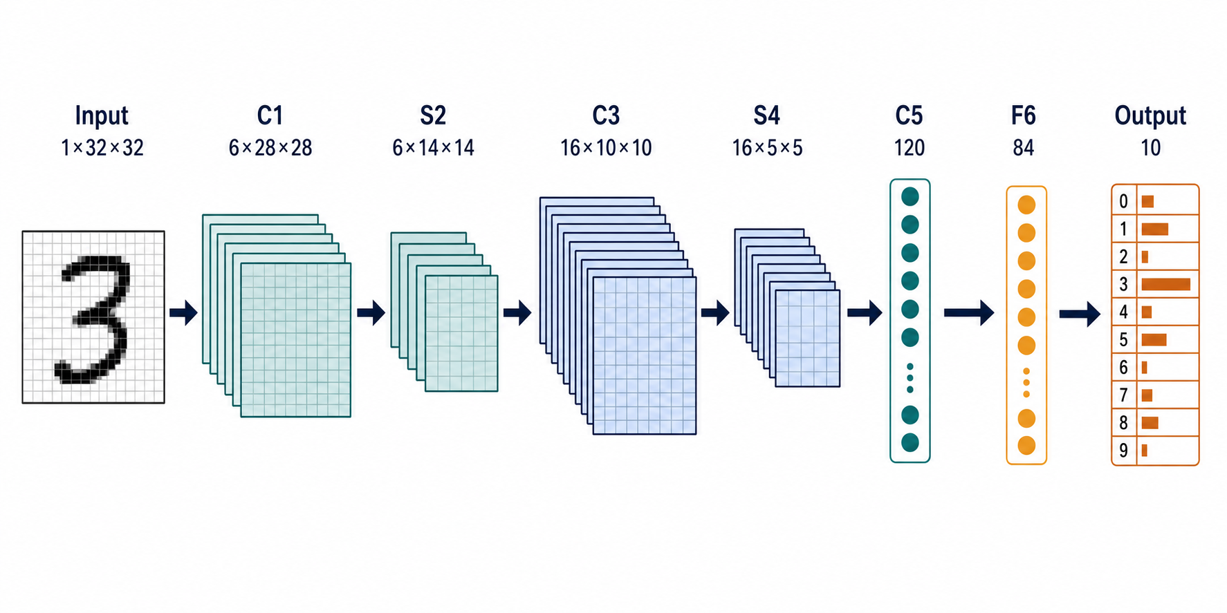
PyTorch 中，image batch 使用 (N, C, H, W) 表示：

N：batch size
C：channel count
H：height
W：width

LeNet 的 input 是 (N, 1, 32, 32)：每个 sample 是一张 32×32 的 grayscale image，1 表示只有一个 channel。

从 input 到 output 的完整 shape 变化：

(N, 1, 32, 32)
→ Conv2d(1, 6, kernel_size=5)
→ (N, 6, 28, 28)
→ Tanh
→ AvgPool2d(kernel_size=2, stride=2)
→ (N, 6, 14, 14)
→ Conv2d(6, 16, kernel_size=5)
→ (N, 16, 10, 10)
→ Tanh
→ AvgPool2d(kernel_size=2, stride=2)
→ (N, 16, 5, 5)
→ Flatten
→ (N, 400)
→ Linear(400, 120)
→ Tanh
→ Linear(120, 84)
→ Tanh
→ Linear(84, 10)
→ (N, 10)

N 在整个网络中不变。真正持续变化的是：

spatial size：32×32 → 28×28 → 14×14 → 10×10 → 5×5
channel count：1 → 6 → 6 → 16 → 16
一维 feature 数量：400 → 120 → 84 → 10

Conv2d 的第一个 5×5 kernel 没有使用 padding，stride 默认是 1，所以输出：

32 - 5 + 1 = 28

第一次 AvgPool2d(2, 2) 使用 2×2 kernel 和 stride=2。每个 2×2 window 只产生一个 value，因此：

28×28 → 14×14

第二组 Conv2d + AvgPool2d 用同样的规则得到：

14×14 → 10×10 → 5×5

最终的 (N, 16, 5, 5) 包含每个 sample 的 16×5×5=400 个 feature value。Flatten 不做计算，只把它整理为 (N, 400)，供后续 Linear 使用。

最后的 (N, 10) 是 10 个 logits，不是 probability。第 k 个 logit 是 model 对 class k 的原始 score。通常将 logits 直接交给 CrossEntropyLoss，而不是在 model 内再手写 Softmax。

与原始 LeNet-5 的差异

我在查询资料时发现，我们现在写的 code 保留了 LeNet 的主干，但并不是对原始 LeNet-5 的逐字复刻。可以看一看这篇：LeNet-5 神经网络结构详解。

S2、S4：Subsampling 不等于当前的 AvgPool2d

原始 LeNet 把 S2、S4 命名为 Subsampling（子采样）。它们都会进行 2×2、stride=2 的 downsampling（下采样），但不只是当前 code 中普通的 AvgPool2d。

对于原始网络的一个 channel，S2/S4 可以近似理解为：

output = Tanh(α × 局部平均值 + β)

其中 α 是 trainable 的缩放 parameter，β 是 trainable bias。

因此原始 S2 有：

6 channels × (1 α + 1 β) = 12 trainable parameters

原始 S4 有：

16 channels × (1 α + 1 β) = 32 trainable parameters

而当前 AvgPool2d(2, 2) 的 trainable parameter 数量是 0。两者都做 downsampling；区别是原始 Subsampling 还能按 channel 调节 output 的缩放和偏移，原始网络在这里存在可学习的参数。

C3：原始 LeNet 使用 partial connection

当前 code 的：

nn.Conv2d(in_channels=6, out_channels=16, kernel_size=5)

表示每一个 output channel 都使用全部 6 个 input channel。parameter 数量为：

16 × (6 × 5 × 5 + 1 bias) = 2416

原始 C3 则使用 partial connection：部分 C3 feature map 只读取 3 个或 4 个 S2 channel，只有最后一个 C3 feature map 读取全部 6 个 channel。它的 parameter 数量是：

6 × (3 × 5 × 5 + 1)
+ 6 × (4 × 5 × 5 + 1)
+ 3 × (4 × 5 × 5 + 1)
+ 1 × (6 × 5 × 5 + 1)
= 1516

这样做可以减少当年的计算量和 parameter 数量，并鼓励不同 C3 feature map 使用不同的 input 组合。这里的“相邻 feature map”只表示 channel index 相邻，不表示 image 中的位置相邻。

C5：Conv2d 与 Linear 在特定 input shape 下等价

原始 C5 的 input 是 16×5×5，kernel size 也是 5×5。每个 C5 unit 会看到：

16 channels × 5 × 5 = 400 input values

它输出 120 个 1×1 feature map，parameter 数量为：

120 × (16 × 5 × 5 + 1 bias) = 48120

当 input spatial size 固定为 5×5 时，这与 Linear(400, 120) 的连接关系相同。因此当前 PyTorch 实现可以先 Flatten，再使用 Linear(400, 120)。

不过它们在 input shape 变大时不一样：Conv2d 仍能滑动并生成更大的 output feature map；Linear 的 input feature 数量被固定为 400。

output layer：RBF 与 logits

原始 LeNet 的 output layer 使用 RBF。它将 F6 的 84-dimensional output 与每个 class 的 84-dimensional template 计算 Euclidean distance。

当前实现使用：

Linear(84, 10) → 10 logits → CrossEntropyLoss

这是现代 PyTorch classification code 更常见的组合。

我的理解

上面的差异至少说明三件事：

1. LeNet 是一个 architecture family 名称，不是一份永远固定的 code。阅读网络时，要继续检查 forward()、layer argument、连接关系和 loss function。
2. Subsampling、AvgPool2d、MaxPool2d 都可能让 spatial size 变小，但实际计算、parameter 数量和保留的信息不同；不能只因为它们的中文名称相近，就把它们当成同一种处理。
3. 原始 C5 在固定 shape 下与 Linear(400, 120) 等价，说明 layer 的名称不如 input-output 连接关系重要。先把 shape 和每个 unit 能看到的 input 搞清楚，才知道两种实现是否真的等价。

用 features 和 classifier 组织 PyTorch code

从 code organization 的角度，把 model 分成 features 和 classifier 两部分是一个很好的习惯。

features：  input image → feature map
classifier：feature map → logits

features 包含两组 Conv2d → Tanh → AvgPool2d：

(N, 1, 32, 32)
→ (N, 6, 28, 28)
→ (N, 6, 14, 14)
→ (N, 16, 10, 10)
→ (N, 16, 5, 5)

classifier 从 Flatten 开始：

(N, 16, 5, 5)
→ (N, 400)
→ (N, 120)
→ (N, 84)
→ (N, 10)

这两个对象不是“两个独立 layer”。它们是两个 nn.Sequential 容器：前者收纳 feature extraction 的 layer，后者收纳 classification 的 layer。这样写让 forward() 只保留网络的总流程：

x = self.features(x)
return self.classifier(x)

下面是 LeNet 网络实现：

import torch
from torch import nn


class LeNet(nn.Module):
    def __init__(self):
        super().__init__()

        # feature extraction
        # 32×32 -> 28×28 -> 14×14 -> 10×10 -> 5×5
        self.features = nn.Sequential(
            # (N, 1, 32, 32) -> (N, 6, 28, 28)
            nn.Conv2d(in_channels=1, out_channels=6, kernel_size=5),
            nn.Tanh(),
            # (N, 6, 28, 28) -> (N, 6, 14, 14)
            nn.AvgPool2d(kernel_size=2, stride=2),
            # (N, 6, 14, 14) -> (N, 16, 10, 10)
            nn.Conv2d(in_channels=6, out_channels=16, kernel_size=5),
            nn.Tanh(),
            # (N, 16, 10, 10) -> (N, 16, 5, 5)
            nn.AvgPool2d(kernel_size=2, stride=2),
        )

        # classification
        self.classifier = nn.Sequential(
            # (N, 16, 5, 5) -> (N, 400)
            nn.Flatten(),
            # 400 -> 120 -> 84 -> 10 logits
            nn.Linear(16 * 5 * 5, 120),
            nn.Tanh(),
            nn.Linear(120, 84),
            nn.Tanh(),
            nn.Linear(84, 10),
        )

    def forward(self, x):
        x = self.features(x)
        return self.classifier(x)


def main():
    model = LeNet()
    
    fake_images = torch.randn(4, 1, 32, 32)
    logits = model(fake_images)

    print(model)
    print(f"input shape: {tuple(fake_images.shape)}")
    print(f"output shape: {tuple(logits.shape)}")

    assert logits.shape == (4, 10)

if __name__ == "__main__":
    main()